
Benchmarking RISC-V: Pre- and Post-Silicon
The XuanTie C906 is currently one of the few RISC-V CPUs that is:
Open-source
RISC-V is an open standard ISA, meaning anyone can implement it without royalties. Unlike GPL software, this does not mean that any distributed implementation also has to be open-source. The majority of the development boards sold today do not provide the RTL source for the CPU :(
Capable of running Linux
Running Linux requires certain features such as privilege modes, (typically) a memory management unit (MMU) and enough memory to fit the kernel and user space programs.
Technically Linux can be configured to function without an MMU, but in our use case that would be a missed opportunity to understand how virtual memory works on a typical modern computer.
Commercially available
Many RISC-V designs exist only as code, are merely emulated in FPGAs, or are only manufactured as a one-time tapeout for academic research.
This makes it an especially interesting platform to tinker with, you can execute programs on a physical board and go all the way down to the CPU’s RTL to understand how it works at every level of abstraction. Well, maybe not at the electron level, but you get the idea.
So I went ahead and bought a development board with one.
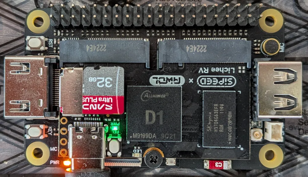
Measuring Operation Latency
Let’s start off easy and try to measure how long a simple instruction such as an add takes.
We can then look at the source code of the CPU and see if it matches our measurement.
Luckily for us, a benchmark suite called lmbench already does this for us.
Note: lmbench source
The original lmbench hasn’t been updated since 2013. I have therefore used Intel’s fork.
$ ./lat_ops
...
integer add: 0.03 nanoseconds
Wait, what? We have a latency of 0.03 ns when a clock cycle is around 0.99 ns? Quite clearly the measurement is wrong, let’s look at lmbench’s source and the resulting executable to see what is going on.
#define TEN(a) a a a a a a a a a a
#define HUNDRED(a) TEN(TEN(a))
...
void
do_integer_add(iter_t iterations, void* cookie)
{
	struct _state *pState = (struct _state*)cookie;
	register int a = pState->N + 57;
	register int b = pState->N + 31;

	while (iterations-- > 0) {
		HUNDRED(a += b; b -= a;)
	}
	use_int(a+b);
}
What is "register"?
The register keyword is a hint to the compiler that these variables should
be kept in registers and not stored in memory. Compilers are free to
ignore it.
0000000000001bd2 <do_integer_add>:
    1bd2:       1141                    addi    sp,sp,-16
    1bd4:       e406                    sd      ra,8(sp)
    1bd6:       4190                    lw      a2,0(a1)
    1bd8:       0396079b                addiw   a5,a2,57
    1bdc:       267d                    addiw   a2,a2,31
    1bde:       cd09                    beqz    a0,1bf8 <do_integer_add+0x26>
    1be0:       fff50713                addi    a4,a0,-1
    1be4:       557d                    li      a0,-1
    1be6:       00f605bb                addw    a1,a2,a5
    1bea:       0007861b                sext.w  a2,a5
    1bee:       9f9d                    subw    a5,a5,a5
    1bf0:       9f8d                    subw    a5,a5,a1
    1bf2:       177d                    addi    a4,a4,-1
    1bf4:       fea719e3                bne     a4,a0,1be6 <do_integer_add+0x14>
    1bf8:       00c7853b                addw    a0,a5,a2
    1bfc:       38b020ef                jal     4786 <use_int>
    1c00:       60a2                    ld      ra,8(sp)
    1c02:       0141                    addi    sp,sp,16
    1c04:       8082                    ret
I don’t think you need to be a math wizard to see that there aren’t two hundred instructions here.
Functions in objdumps
The first two lines and the last three lines here are fairly standard.
addi    sp,sp,-16     # Subtract 16 from the stack pointer
sd      ra,8(sp)      # Save value in return address register
                      # to (the address in sp) + 8 bytes
...
ld      ra,8(sp)      # Restore return address back to ra register
addi    sp,sp,16      # Restore stack pointer to original value
ret                   # Return from function call
It starts off by allocating space for local variables and any registers that need to be saved. With a stack this is easy, just a simple decrement from the stack pointer, as most modern architectures use a downward-growing stack.
Since we have a jal inside our function (a call to use_int),
we are overwriting the ra register. We therefore have to save it
so that we can restore it before calling ret.
Function arguments are stored in a0-a7 by the caller before the jump.
If more than 8 arguments are passed, the remaining ones are stored in the stack.
In our case a0 is iterations and a1 is cookie. We ourselves
overwrite a0 with a + b (a5 + a2) just before calling use_int.
The interesting part is the lines between beqz and bne, this is the inner
loop that is supposed to have a hundred a += b; b -= a; instructions.
The authors have tried to prevent this from being optimized by making the
two operations depend on the results of each other, and also by using
the final results in use_int(a+b). It looks like compilers have
gotten a lot smarter since then, and this has been compressed
into just four (pseudo)instructions:
addw    a1,a2,a5  # tmp = b + a
sext.w  a2,a5     # b = a
subw    a5,a5,a5  # a = 0
subw    a5,a5,a1  # a = - tmp
At the end we get
b = a
a = - a - b
The reason that the instructions look weird is that int on RISC-V Linux
is 32 bits so sign extension has to be performed. But is the final result really correct??
As a sanity check let’s try it out.
a = 123
b = 321

for i in range(100):
    a += b
    b -= a

print(a) # -444
print(b) # 123
Just goes to show how good compilers have become at optimizing equations. We can prevent this from being optimized away by telling the compiler that we are using the values between the operations.
// HUNDRED(a += b; b -= a;)
HUNDRED(a += b;
        __asm__ volatile("" : "+r"(a), "+r"(b));
        b -= a;
        __asm__ volatile("" : "+r"(a), "+r"(b));
)
The first argument inside _asm_ is empty, meaning that
we haven’t actually provided any new assembly instructions.
We are just telling the compiler that a and b need to be
treated as if they are being read from and written into.
The intermediate values therefore can not be optimized away.
The volatile keyword prevents the _asm_ section itself
from being optimized away.
Let’s recompile and look at the objdump again.
0000000000001888 <do_integer_add>:
    ...
    18a2:       9d3d                    addw    a0,a0,a5
    18a4:       9f89                    subw    a5,a5,a0
    18a6:       9d3d                    addw    a0,a0,a5
    18a8:       9f89                    subw    a5,a5,a0
    18aa:       9d3d                    addw    a0,a0,a5
    18ac:       9f89                    subw    a5,a5,a0
    18ae:       9d3d                    addw    a0,a0,a5
    18b0:       9f89                    subw    a5,a5,a0
    18b2:       9d3d                    addw    a0,a0,a5
    18b4:       9f89                    subw    a5,a5,a0
    ...
Now we can re-run and try again.
$ ./lat_ops
...
integer add: 1.04 nanoseconds
How do computers keep track of time anyway?
With the help of hardware. In RISC-V, the “Zicntr” extension
defines a time register that is updated relative to “wall clock” time,
meaning that it corresponds to actual time passed like a clock on the wall.
The value itself is not meaningful, the kernel has to look at the difference
at different measurement points to determine how much time has passed and increment the
system clock accordingly. Similar registers exist in other architectures.
This value is updated with a hardware counter from outside the CPU. The hardware takes a constant frequency clock, typically separate from the CPU. The circuits used to generate clocks are called the clock oscillator and the phase-locked loop. But at this point we are no longer in the purely digital realm.
For the XuanTie C906, the time register is updated from outside
via the pad_cpu_sys_cnt pad.
When incrementing the system clock, the kernel also has to divide the difference by the tick rate. In RISC-V, this information is provided in the device tree files found in the kernel’s source code.
# arch/riscv/boot/dts/allwinner/sun20i-d1s.dtsi
timebase-frequency = <24000000>;
...
opp-hz = /bits/ 64 <1008000000>;
So our CPU usually runs at 1 GHz whereas the timer runs at 24 MHz. Even though Linux’s system clock has a granularity of 1 ns, we are measuring with a granularity of around 42 ns.
Our clock period is around 0.99 ns, so apparently an add instruction takes one clock cycle and we have a measurement overhead of around 0.05 ns. Is this accurate? Since we have access to the source code of the CPU, we can take the same loop used in the benchmark and run it in a simulation, allowing us to examine every signal. How neat is that!
Back to RTL
There are two things I’d like to see in simulation: The complete path
a single add instruction takes, and a bunch of adds back-to-back
like in lmbench. You can view the source code here.
Note that we are simulating our program running
on bare metal. The MMU is skipped here, and our virtual addresses
are the same as physical addresses.
The CPU starts off by fetching the instruction, performed by the instruction fetch unit (IFU). It first looks in its 32 KB instruction cache. The cache is made up of four 32-bit banks in parallel, each consisting of 2048 rows.
What do you mean by "banks"? Why four in parallel?
Companies provide SRAM macros that can actually be manufactured by a specific foundry process and are optimized for various metrics (area, latency, power, dual-port reads/writes etc.). These are provided in specific sizes. If your design needs a larger width, you can combine multiple in parallel.
Let’s talk about how the IFU checks if an instruction at an address has been cached.
The CPU is 64-bit, so we are working with 64-bit addresses. Even though the MMU is skipped, the CPU is still designed to use the Sv39 virtual addressing scheme. This means the upper 25 bits aren’t used.
Virtual Addresses? MMU? What is all that?
Operating systems (with the help of hardware) provide an illusion of large address space to each running program, so that software engineers don’t have to worry about other programs interfering with their address space. The addresses each program sees are actually virtual addresses. The mapping to physical addresses in memory is cached in the translation lookaside buffer (TLB) inside the MMU. Read more about it in Operating Systems: Three Easy Pieces, chapters 12 to 24, freely available online.
The cache line is 64 bytes, meaning that an entry stores 64 bytes of instructions. Since the SRAM blocks are a total of 16 bytes wide, 4 separate writes are needed for each entry. Couldn’t they have used even more banks in parallel to achieve this in a single parallel write? They could have, but shallow and wide SRAMs tend to be inefficient, sacrificing a metric like area. Besides, requested reads are only 8 bytes anyway.
Bits 5:0 of the address are used to determine where in the 64-byte
entry we are requesting.
Bits 13:6 are used for the row (tag index), in other words where in the
cache to store our instructions. What about all the other addresses
that share those bits, how does the cache tell them apart?
Bits 39:12 are used for the tag, the cache stores this
in a separate 256x59 bank, along with a valid bit.
Yes, some of the tag overlaps with the tag index.
I don’t know why.
Perhaps something to do with paging when the MMU is enabled,
but that’s for another day.
If this tag matches, and the valid bit is set, then the address is cached.
The cache is 2-way, meaning that it can store two entries (and tags) for
each tag index. Both are checked at the same time.
That is a total of 256 sets x 64 B x 2-way = 32 KB.
Our first add instruction is in location 0x6f8
 6f4:	0001                	nop
 6f6:	0001                	nop
 6f8:	006283b3          	add	t2,t0,t1
 6fc:	0001                	nop
 6fe:	0001                	nop
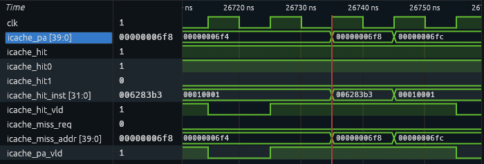
The IFU checks address 0x6f8 in the cache for the
first time at time 26735 ns, and it’s a hit!
Looks like it was pre-fetched earlier.
Let’s figure out when it was actually requested
from memory.
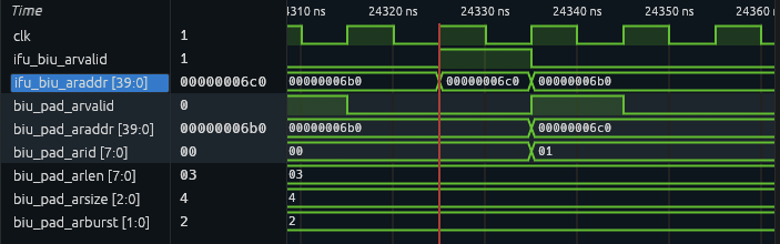
The read request originates in the IFU at time 24325 ns and is forwarded to the bus interface unit (BIU). The simulated memory won’t have the same characteristics as actual DRAM, it’s possible that in reality the instruction wouldn’t be pre-fetched in time.
After fetching the instruction, the CPU has to decode it in the instruction decode unit (IDU). It’s also in this stage that we read from registers.
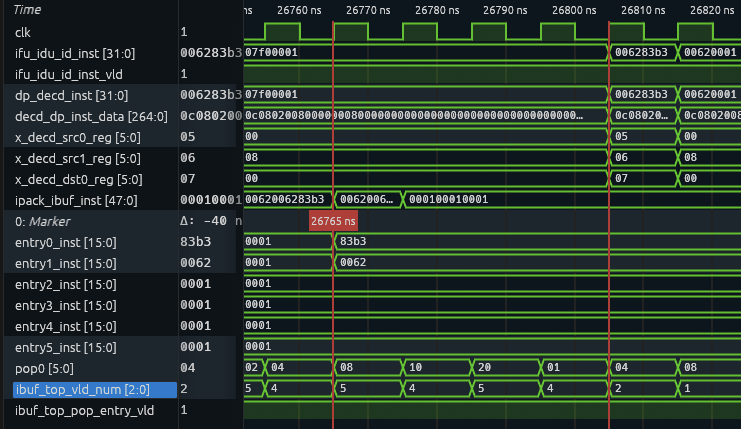
The instruction 0x6283b3 is passed to the IDU
from the IFU via a ring buffer. The ring buffer consists
of six 4-byte entries, being able to fit six compressed
instructions or three standard ones. Our add arrives
at the ring buffer at 26765 ns. The other entries in the
ring buffer contain the compressed nop instruction 0x0001.
Our add is popped from the ring buffer into the IDU
at 26805 ns, and is decoded instantly.
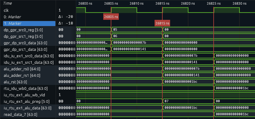
Data in the register source is also read as soon as the instruction
is popped from the ring buffer into the IDU. In the next clock cycle,
the instruction is forwarded to the instruction unit (IU). The
adder inside the arithmetic logic unit (ALU) performs the addition
instantly. The writeback to the result register is also initiated instantly,
and the result is available to be read in the next clock cycle.
At time 26825 ns, our add is finally complete!
Does this match what we measured in hardware?
The term “latency” is not very meaningful without defining the specific
start and end points. If we measure from the moment the instruction
is fetched from cache to the moment the result is written back
to a register, the latency we measured is (26825 - 26735) / 10 = 9
clock cycles. If we start from the moment an instruction arrives at the
IDU to the moment it is written back to a register, it is (26825 - 26805) / 10 = 2
clock cycles. If we just measure from the moment the instruction arrives at the
IU to the register writeback, it’s only (26825 - 26815) / 10 = 1 cycle.
Let’s take a look at what happens when it performs many adds back-to-back.
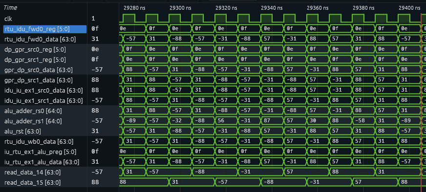
The processor is pipelined so we are seeing an add/sub executed every cycle.
We can also see that the values return to their original values every 12 cycles (6 inner loops),
which is why the compiler was able to optimize away earlier.
How Does lmbench Measure Latency?
Before starting the measurement, lmbench performs a warmup and calculates how many iterations to run the benchmark for. The purpose of this is to reduce measurement overhead.
How does the warmup lower overhead?
By requesting access to data before we actually do anything useful with it, we can fill up our caches and the TLB with the data we will actually need. This is a common latency optimization technique called cache warming.
There are also other benefits, such as providing historical information to the branch predictor, which can then be used in its predictions.
Keep in mind that lmbench is a benchmark suite, and
that other more complicated benchmarks may benefit more from this
than a simple add latency measurement.
It calculates how many iterations are required to run the
benchmark for one second by first finding
“smallest timing interval that has accurate timing”.
This is done by checking if the iteration count and the runtime scale almost linearly with small differences.
It then scales the iteration count to be enough to run for one second,
and measures the runtime of this iteration count repetitions times, where
repetitions is an optional user-supplied argument, or 11 by default.
To get the latency of an individual operation, it has to divide
the measured time by the iteration count times the amount of
operations inside one iteration (100 adds + 100 subs in integer add).
The final result reported is the median of the repetitions measurements.
We can get a tiny bit closer to the simulated measurement of 1 clock cycle (0.99 ns) by printing out the smallest measurement instead of the median.
integer add: 1.03 nanoseconds
And another tiny bit further by increasing the operation count in a single loop from 200 to 2000, decreasing the overhead of the loop.
integer add: 1.02 nanoseconds
But increase the operation count too far, for example to 20000, and now we have 20000 x 4 B = 80000 B of instructions, which no longer fits into our 32 KB instruction cache. The warmup step can’t save us anymore.
integer add: 2.43 nanoseconds
Ouch! Cache misses are costly.
One second is quite a long time for a modern CPU. It’s quite difficult
to measure 0.99 ns because the kernel will perform context switches
and run other programs during our benchmark. It is possible to configure
Linux to avoid scheduling user programs on specific cores, but our CPU
is single-core so that is not an option for us. Besides, kernel code
can still run on these, so we probably still wouldn’t measure 0.99 ns.
Running with higher priority using nice -20 didn’t result in a
further drop. I also tried chrt -f 99, but I can’t ssh back into
the machine to see the results after that without rebooting first.
Redirecting output to a file didn’t work either.
What About Other Instructions?
As a final test, let’s measure how long a mul takes on real hardware
and in simulation.
integer mul: 3.20 nanoseconds
So three clock cycles, plus overhead. Does that match simulation results?
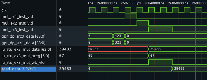
So the multiplier has three stages and initiates the register
writeback 2 cycles after receiving the instruction.
Unlike the add case, the result isn’t available to be read
from the register in the next cycle, but rather 2 cycles after,
totaling a 4-cycle latency. It appears that writeback can take
1 or 2 cycles, perhaps explaining why the hardware measurement
wasn’t closer to 3 ns.
Closing thoughts
While having access to a physical CPU along with its source is really exciting, the experience has also been quite frustrating. I’ve had to deal with:
- Buggy Wi-Fi drivers that I had to manually patch using fixes found in newer kernel versions not available in Ubuntu repositories yet
- Mystery chinese executables with no source code
- Files hosted on Baidu and MEGA
- Tutorials found in text files that just contain a broken link to what appears to have once been a forum thread alongside “You can read it using Google Translate”.
I also would’ve liked to simulate Linux running with the exact same binaries, this would’ve allowed me to compare so much more than just instruction latency, such as latencies of syscalls and context switches. Unfortunately only the CPU is open-source, the rest of the SoC is not, meaning that I can’t take the same Ubuntu I installed on hardware and simulate it. I could try building my own SoC with a project like litex, and others have gotten Linux running in simulation on other open-source RISC-V CPUs with litex, but at that point the results won’t match our actual hardware.
It really is a shame, a completely open-source SoC (that is also commercially available and capable of running modern Linux distros) with better documentation would be an invaluable educational resource for universities and tinkerers. Maybe one of the readers could run off with that business idea.
Thank you for reading this far. If you have any feedback or suggestions, please contact me via email or on LinkedIn.